
Sequence-to-sequence learning with Transducers
Published:
The Transducer (sometimes called the “RNN Transducer” or “RNN-T”, though it need not use RNNs) is a sequence-to-sequence model proposed by Alex Graves in “Sequence Transduction with Recurrent Neural Networks”. The paper was published at the ICML 2012 Workshop on Representation Learning. Graves showed that the Transducer was a sensible model to use for speech recognition, achieving good results on a small dataset (TIMIT).
Since then, the Transducer hasn’t been used as much compared to CTC models (like Deep Speech 2) or attention models (like Listen, Attend, and Spell). Last year, however, the Transducer got some serious attention when Google researchers showed that it could enable entirely on-device low-latency speech recognition for Pixel phones. And more recently, the Transducer was used to achieve a new state-of-the-art word error rate for the LibriSpeech benchmark.1
So what is the Transducer, and when might you want to use it? In this post, we will see where Transducer models fit in with other sequence-to-sequence models and a detailed explanation of how they work.
This post also includes a Colab notebook with a PyTorch implementation of the Transducer for a toy problem—which you can skip straight to here.
Attention models
The problems we’re interested in here are sequence transduction problems, where the goal is to map an input sequence $\mathbf{x} = \{x_1, x_2, \dots x_T\}$ to an output sequence $\mathbf{y} = \{y_1, y_2, \dots, y_U\}$.
The go-to models for sequence transduction problems are attention-based sequence-to-sequence models, like RNN encoder-decoder models or Transformers.
Here’s a diagram of an attention model. (In the diagrams below, I’ll use red to indicate that a module has access to $\mathbf{x}$, blue to indicate access to $\mathbf{y}$, and purple to indicate access to both $\mathbf{x}$ and $\mathbf{y}$.)
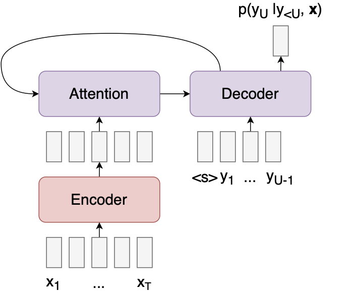
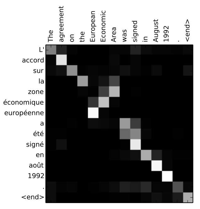
The model encodes the input $\mathbf{x}$ into a sequence of feature vectors, then computes the probability of the next output $y_u$ as a function of the encoded input and previous outputs. The attention mechanism allows the decoder to look at different parts of the input sequence when predicting each output. Here, for example, is a heatmap of where the decoder is looking during a translation task (from Bahdanau et al.):
Attention models can be applied to any problem, but they are not always the best choice for certain problems, like speech recognition, for a few reasons2:
- The attention operation is expensive for long input sequences. The complexity of attending to the entire input for every output is $O(TU)$—and for audio, $T$ and $U$ are big.
- Attention models cannot be run online (in real time), since the entire input sequence needs to be available before the decoder can attend to it.
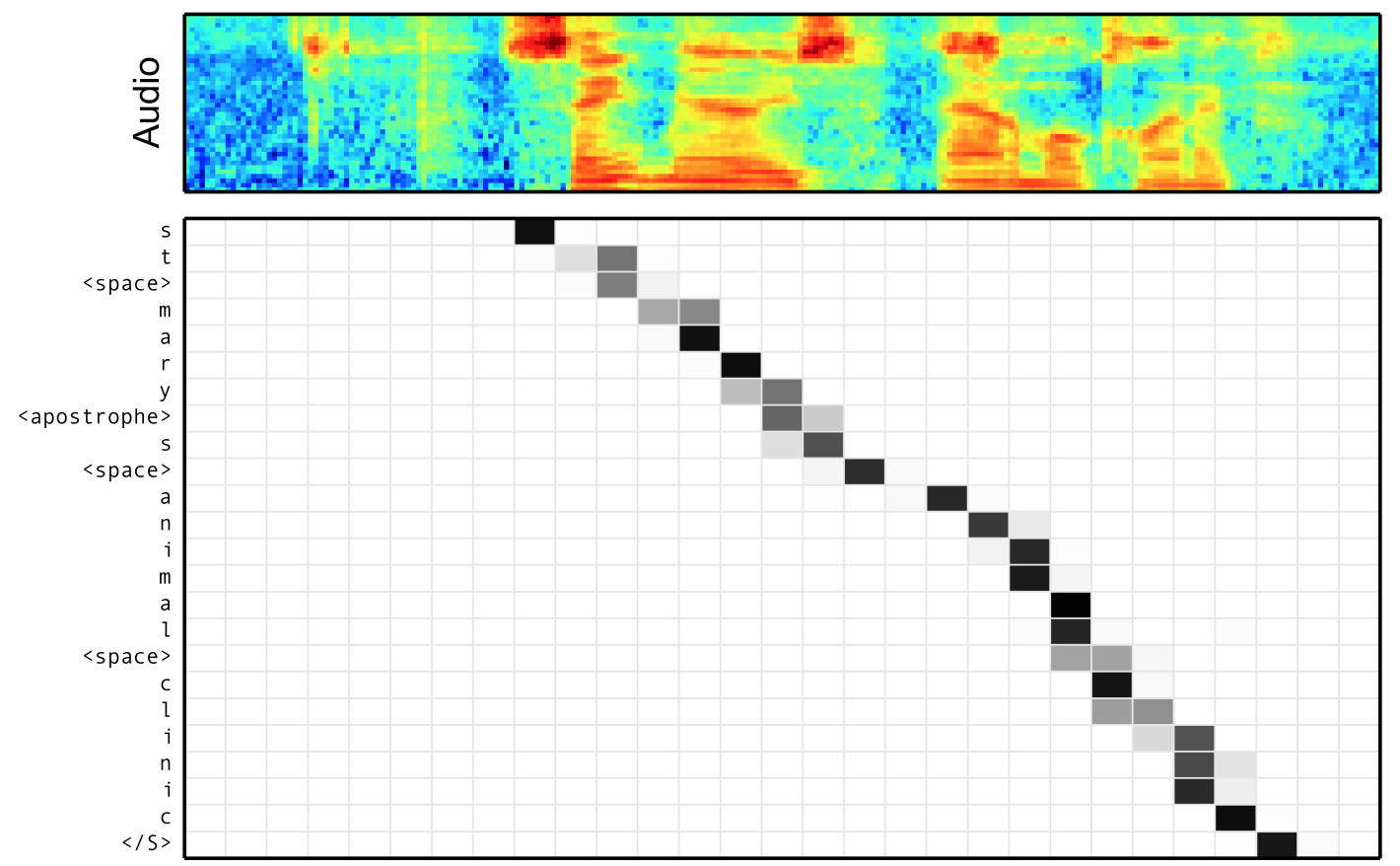
- Attention models also don’t take advantage of the fact that, for speech recognition, the alignment between inputs and outputs is monotonic: that is, if word A comes after word B in the transcript, word A must come after word B in the audio signal (see image below, from Chan et al., for an example of a monotonic alignment). The fact that attention models lack this inductive bias seems to make them harder to train for speech recognition; it’s common to add auxiliary loss terms to stabilize training.
This leads us to Connectionist Temporal Classification (CTC) models, which are more suitable for some problems than attention models.
CTC models
CTC models assume that there is a monotonic input-output alignment3. This ends up making the model a lot simpler.
So simple! We only need a single neural net to implement a CTC model, and no expensive global attention mechanism.
But CTC models have a couple problems of their own:
- Problem 1: The output sequence length $U$ has to be smaller than the input sequence length $T$. This might not seem like a problem for speech recognition, where $T$ is much larger than $U$—but it prevents us from using a model architecture that does a lot of pooling, which can make the model a lot faster.
- Problem 2: The outputs are assumed to be independent of each other. The result is that CTC models often produce outputs that are obviously wrong, like “I eight food” instead of “I ate food”. Getting good results with CTC usually requires a search algorithm that incorporates a secondary language model.4
Can we do better than CTC? Yes: using Transducer models.
Transducer models
The Transducer elegantly solves both problems associated with CTC, while retaining some of its advantages over attention models.
- It solves Problem 1 by allowing multiple outputs for each input.
- It solves Problem 2 by adding a predictor network and joiner5 network.
The predictor is autoregressive: it takes as input the previous outputs and produces features that can be used for predicting the next output, like a standard language model.
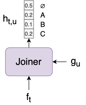
The joiner is a simple feedforward network that combines the encoder vector $f_t$ and predictor vector $g_u$ and outputs a softmax $h_{t,u}$ over all the labels, as well as a “null” output $\varnothing$.
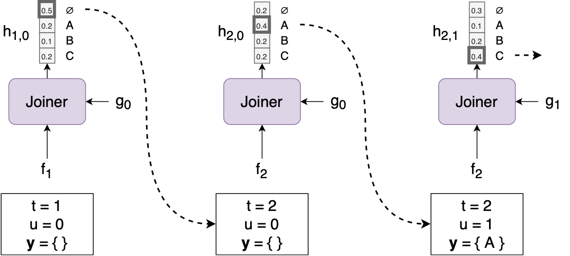
Given an input sequence $\mathbf{x}$, generating an output sequence $\mathbf{y}$ can be done using a simple greedy search algorithm:
Start by setting $t := 1$, $u := 0$, and $\mathbf{y} :=$ an empty list.
Compute $f_t$ using $\mathbf{x}$ and $g_u$ using $\mathbf{y}$.
Compute $h_{t,u}$ using $f_t$ and $g_u$.
If the argmax of $h_{t,u}$ is a label, set $u := u + 1$, and output the label (append it to $\mathbf{y}$ and feed it back into the predictor).
If the argmax of $h_{t,u}$ is $\varnothing$, set $t := t + 1$ (in other words, just move to the next input timestep and output nothing).If $t=T+1$, we’re done. Else, go back to step 2.
A couple cool things about Transducers to note here:
If the encoder is causal (i.e., we’re not using something like a bidirectional RNN), then the search can run in an online/streaming fashion, where we process each $x_t$ as soon as it arrives.
The predictor only has access to $\mathbf{y}$, and not $\mathbf{x}$—unlike the decoder in an attention model, which sees both $\mathbf{x}$ and $\mathbf{y}$. That means we can easily pre-train the predictor on text-only data, which there’s a lot more of than paired (speech, text) data.
Alignment
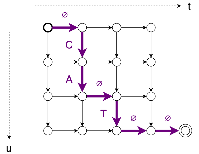
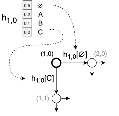
Given an $(\mathbf{x}, \mathbf{y})$ pair, the Transducer defines a set of possible monotonic alignments between $\mathbf{x}$ and $\mathbf{y}$. For example, consider an input sequence of length $T = 4$ and an output sequence (“CAT”) of length $U = 3$. We can illustrate the set of alignments using a graph6 like this:
Here’s one alignment: $\mathbf{z} = \varnothing, C, A, \varnothing, T, \varnothing, \varnothing$
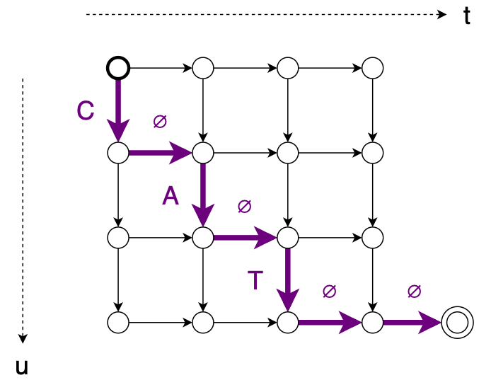
Here’s another alignment: $\mathbf{z} = C, \varnothing, A, \varnothing, T, \varnothing, \varnothing$
We can calculate the probability of one of these alignments by multiplying together the values of each edge along the path:
$\mathbf{z} = \varnothing, C, A, \varnothing, T, \varnothing, \varnothing$
↓ $p(\mathbf{z} | \mathbf{x}) = h_{1,0}[\varnothing] \cdot h_{2,0}[C] \cdot h_{2,1}[A] \cdot h_{2,2}[\varnothing] \cdot h_{3,2}[T] \cdot h_{3,3}[\varnothing] \cdot h_{4,3}[\varnothing],$
where the value of an edge is the corresponding entry of $h_{t,u}$.
Training
How do we train the model? If we knew the true alignment7 $\mathbf{z}$, we could minimize the cross-entropy between $\mathbf{h}$ and $\mathbf{z}$, like a normal classifier. However, we usually don’t know the true alignment (and for some tasks, a “true” alignment might not even exist).
Instead, the Transducer defines $p(\mathbf{y}|\mathbf{x})$ as the sum of the probabilities of all possible alignments between $\mathbf{x}$ and $\mathbf{y}$. We train the model by minimizing the loss function $-\log p(\mathbf{y}|\mathbf{x})$.
There are usually too many possible alignments to compute the loss function by just adding them all up directly. To compute the sum efficiently, we compute the “forward variable” $\alpha_{t,u}$, for $1 \leq t \leq T$ and $0 \leq u \leq U$:
We can visualize this computation as passing values along the edges of the alignment graph:
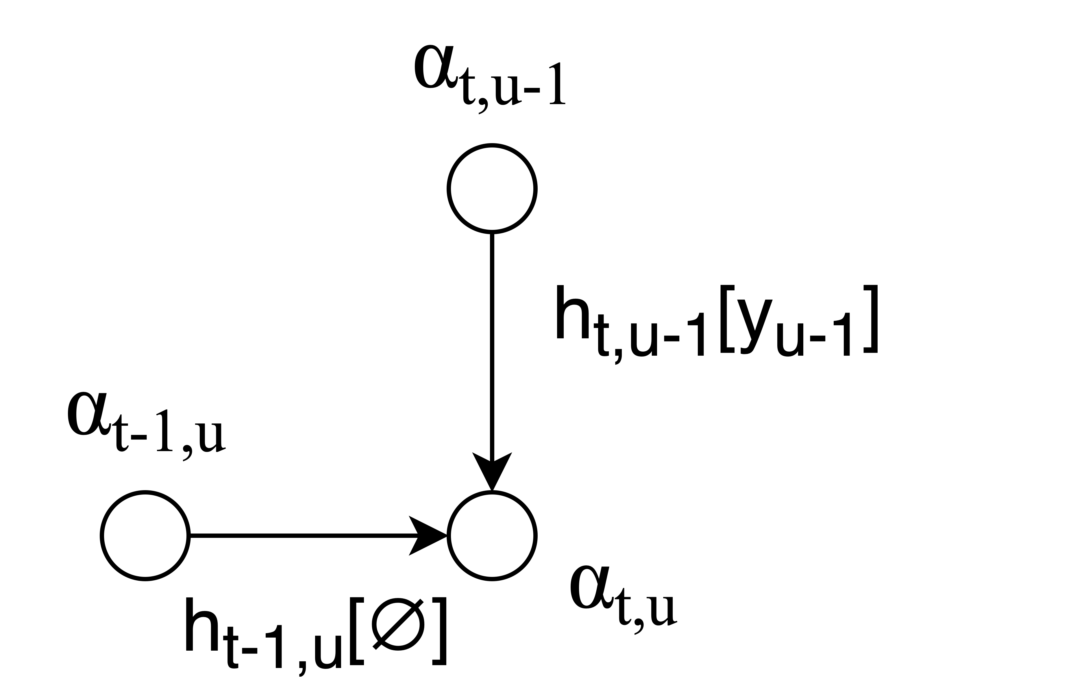
After we’ve computed $\alpha_{t,u}$ for every node in the alignment graph, we get $p(\mathbf{y}|\mathbf{x})$ using the forward variable at the last node of the graph:
We need to do everything in the log domain, for the usual reasons. In the log domain, the computation becomes:
Finally, to compute the gradient of the loss $-\log p(\mathbf{y}|\mathbf{x})$, there is a second algorithm that computes a backward variable $\beta_{t,u}$, using the same computation as $\alpha_{t,u}$, but in reverse, starting from the last node.
In the notebook, I provide a simple PyTorch implementation of the loss function that only writes out the forward computation and uses automatic differentiation to compute the gradient. This is a lot slower than a lower-level implementation, but easier to program and to read.
Memory usage
In general, Transducer models seem like a good idea. But here’s the catch (and possibly the unspoken reason that the Transducer never caught on until recently):
Suppose we have $T=1000$, $U=100$, $L=1000$ labels, and batch size $B=32$. Then to store $h_{t,u}$ for all $(t,u)$ to run the forward-backward algorithm, we need a tensor of size $B \times T \times U \times L = $ 3,200,000,000, or 12.8 GB if we’re using single-precision floats. And that’s just the output tensor: there’s also the hidden unit activations of the joiner network, which are of size $B \times T \times U \times d_{\text{joiner}}$.
So unless you are, ahem, a certain tech company in possession of TPUs with plentiful RAM (guess who’s been publishing the most Transducer papers!), you may need to find some way to reduce memory consumption during training—e.g., by pooling in the encoder to reduce $T$, or by using a small batch size $B$.
Ironically, this is only a problem during training; during inference, we only need a small amount of memory to store the current activations and hypotheses for $\mathbf{y}$.
Search
We saw earlier that you can predict $\mathbf{y}$ using a greedy search, always picking the top output of $h_{t,u}$. Better results can be obtained using a beam search instead, maintaining a list of multiple hypotheses for $\mathbf{y}$ and updating them at each input timestep.
The Transducer beam search algorithm can be found in the original paper—though it is somewhat gnarlier than the simple attention model beam search, and I confess I haven’t implemented it myself yet. (Check out the soon-to-be-released SpeechBrain toolkit for my colleagues’ implementation.)
Code
Finally, the Colab notebook for the Transducer can be found here. The notebook implements a Transducer model in PyTorch for a toy sequence transduction problem (filling in missing vowels in a sentence: “hll wrld” –> “hello world”), including the loss function, the greedy search, and a function for computing the probability of a single alignment. Enjoy!
Citation
If you found this tutorial helpful and would like to cite it, you can use the following BibTeX entry:
@misc{
	lugosch_2020,
	title={Sequence-to-sequence learning with Transducers},
	url={https://lorenlugosch.github.io/posts/2020/11/transducer/},
	author={Lugosch, Loren},
	year={2020},
	month={Nov}
}
It always seems to take a few years between Alex Graves publishing a good idea and the research community fully recognizing it. There was an 8 year gap between CTC (2006) and Baidu’s Deep Speech (2014), and an 8 year gap between the Transducer (2012) and Google’s latest result (2020). This suggests a simple algorithm for achieving state-of-the-art results: select a paper written by Alex Graves from 8 years ago, and reimplement it using whatever advances in deep learning have been made since then. Maybe 2022 will be the year Neural Turing Machines really shine! ↩
There’s been some interesting work developing attention models that do not have these three issues, like monotonic chunkwise attention (MoChA). ↩
As do their older cousins, Hidden Markov Models, Graph Transformer Networks, and the more recent AutoSegCriterion. See Awni Hannun’s excellent introduction if you want to learn more about CTC. ↩
Alternately, you can use a very big and deep network like Jasper. Jasper was a CTC model proposed by NVIDIA researchers that, astonishingly, achieved nearly state-of-the-art performance using only a greedy search. If the model is big and deep, it can intelligently coordinate its outputs so as to not produce dumb predictions like “I eight food” instead of “I ate food”. Still, it seems to be more parameter-efficient to use a model that explicitly assumes that outputs are not independent, like attention models and Transducer models. ↩
In the original paper, there was no joiner; the encoder vector and predictor vector were simply added together. Graves and his co-authors added the joiner in a subsequent paper, finding that it reduced the number of deletion errors. ↩
If you’re familiar with the powerful gadgets known as finite state transducers (FSTs), you may recognize that the Transducer graph is a weighted FST, where an alignment forms the input labels, $\mathbf{y}$ forms the output labels, and the weight for each edge is dynamically generated by the joiner network. ↩
The true alignment of neural networks is known to be Chaotic Good. ↩