An introduction to sequence-to-sequence learning

Many interesting problems in artificial intelligence can be described in the following way:

Map a sequence of inputs $\mathbf{x}$ to the correct sequence of outputs $\mathbf{y}$.

Speech recognition is one example: the goal is to map an audio signal $\mathbf{x}$ (a sequence of real-valued audio samples) to the correct text transcript $\mathbf{y}$ (a sequence of letters). Other examples are machine translation, image captioning, and speech synthesis.

This post is a tutorial introduction to sequence-to-sequence learning, a method for using neural networks to solve these “sequence transduction” problems. In this post, I will:

• show you why these problems are interesting and challenging
• give a detailed description of sequence-to-sequence learning—or “seq2seq”, as the cool kids call it
• walk through an example seq2seq application (with PyTorch code)

The only background you need to read this is basic knowledge of how to train and use neural networks for classification problems.

The problem

Let’s start by defining the general problem of sequence transduction a little more carefully.

Let $\mathbf{x} = \{x_1, x_2, \dots x_T\}$ be the input sequence and $\mathbf{y} = \{y_1, y_2, \dots, y_U\}$ be the output sequence, where $x_t \in \mathcal{S}_x$, $y_u \in \mathcal{S}_y$, and $\mathcal{S}_x$ and $\mathcal{S}_y$ are the sets of possible things that each $x_t$ and $y_u$ can be, respectively.

In speech recognition, $\mathcal{S}_x$ would be the set of real numbers, $\mathcal{S}_y$ would be the set of letters, $T$ might be on the order of thousands, and $U$ might be on the order of tens.

We’ll assume that the inputs and outputs are random variables, and the value of $T$ and $U$ may vary between examples of $\mathbf{x}$ and $\mathbf{y}$—for example, not all sentences have the same length. The fact that $U$ may vary is part of what makes these problems challenging: we need to guess how long the output should be, and often this can’t simply be inferred from the input length.

The goal is to find the best function $f(\mathbf{x})$ for mapping $\mathbf{x}$ to $\mathbf{y}$. But what does “best” mean here?

For a classification problem, the “best” $f(\mathbf{x})$ is the one with the highest accuracy, i.e. the lowest probability of guessing an output $\mathbf{\hat{y}}$ which is not equal to the true $\mathbf{y}$.

Similarly, we can use “accuracy” as a performance measure if the output is a sequence: if the guess $\mathbf{\hat{y}}$ is at all different from the true output $\mathbf{y}$, the output is incorrect. That is, if $\mathbf{y} = \text{“hello”}$ and $\mathbf{\hat{y}} = \text{“helo”}$, then $\mathbf{\hat{y}}$ is incorrect. This is also called the “$0$-$1$ loss”: $0$ if $\mathbf{\hat{y}} = \mathbf{y}$, $1$ otherwise.

The simple $0$-$1$ loss is not a realistic performance measure: an output like $\text{“lskdjfl”}$ should really be regarded as less accurate than $\text{“helo”}$ if the true output is $\text{“hello”}$.

In practice, we probably care more about some other performance measure, such as the word error rate (speech recognition) or the BLEU score (machine translation, image captioning). But the $0$-$1$ loss is often a good approximation or surrogate for other performance measures, and it doesn’t require any domain-specific knowledge to apply, so let’s assume that the $0$-$1$ loss is what we’re trying to optimize.

The ideal solution

Suppose that we have access to a magical genie who can tell us $p(\mathbf{y}|\mathbf{x})$, the probability that the correct output sequence is $\mathbf{y}$ given that the input is $\mathbf{x}$, for any $\mathbf{x}$ and $\mathbf{y}$. In that case, what would be the best function $f(\mathbf{x})$ to use?

Since we’re trying to minimize the probability of making an error (guessing a $\mathbf{\hat{y}}$ which is not equal to the correct $\mathbf{y}$), the following function is the best choice:

Alas! We usually don’t have a magical genie who can tell us $p(\mathbf{y}|\mathbf{x})$. What we can do instead is fit a model $p_{\theta}(\mathbf{y}|\mathbf{x})$ to some training data, and if we’re lucky, that model will be close to the true distribution $p(\mathbf{y}|\mathbf{x})$.

Modeling $p(\mathbf{y})$

Before we consider implementing the model $p_{\theta}(\mathbf{y}|\mathbf{x})$, let’s start with a slightly easier but closely related problem: implementing a model $p_{\theta}(\mathbf{y})$ that is close to $p(\mathbf{y})$.

What $p(\mathbf{y})$ represents is the probability of observing a particular output sequence $\mathbf{y}$, independent of whatever the input sequence might be.

Intuitively, what does this mean? Well, consider the two following sequences of words:

The probability of observing $\mathbf{y}_1$ should be higher than the probability of observing $\mathbf{y}_2$, since $\mathbf{y}_1$ is a meaningful English sentence, and $\mathbf{y}_2$ is nonsensical. This fact could be useful in speech recognition to figure out which of the two phrases the person actually said, since both of these phrases sound the same if you say them out loud.

Likewise, consider the two following sequences of letters:

Although these two sequences are both not real English words, the first one $\mathbf{y}_1$ really could be an English word, whereas the second one $\mathbf{y}_2$ just looks like someone banging on a keyboard. If we were to train a model $p_{\theta}(\mathbf{y})$ on English text, we would probably find in this case that $p_{\theta}(\mathbf{y}_1) > p_{\theta}(\mathbf{y}_2)$.

To assign a probability to any sequence, we could just use a gigantic lookup table, with one entry for every possible $\mathbf{y}$. The problem is there are usually too many possible sequences for this to be feasible—in fact, there may be infinitely many possible sequences.

Instead, let’s define a model that computes the probability of a sequence by dividing it into a number of simpler probabilities using the chain rule of probability.

The chain rule of probability says that, for two random variables A and B, the probability of A and B is equal to the probability of A given B, multiplied by the probability of B:

That’s one way to factorize $p(A,B)$—we could also factorize it like this:

Moreover, you can apply the chain rule for as many random variables as you want:

Remember that our sequence $\mathbf{y}$ is a collection of random variables $y_1, y_2, y_3, \dots, y_U$. So let’s use the chain rule to write out $p_{\theta}(\mathbf{y})$ as the product of the probability of each of these variables, given the previous ones:

This $p_{\theta}(y_u|y_{u-1},y_{u-2},\dots,y_{1})$ term means “the probability of the next element, given what came before”. A model that implements $p_{\theta}(y_u|y_{u-1},y_{u-2},\dots,y_{1})$ is sometimes called a “next step predictor” or “language model”. When you are texting someone, and your phone suggests the next word for you as you are typing, it uses a model like this.

We can implement this “next step” probability $p_{\theta}(y_u|y_{u-1},y_{u-2},\dots,y_{1})$ using a neural network¹. The neural network takes as input the previous $y_u$’s and predicts the next $y_u$. This is shown in the figure below:

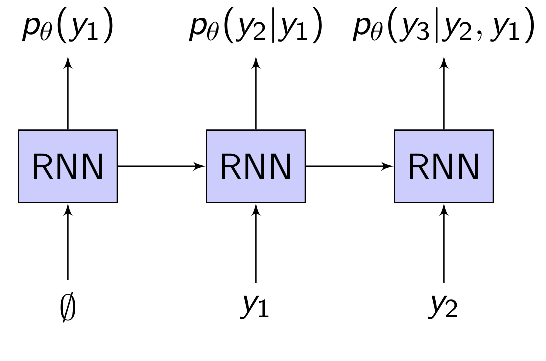
For example, if $\mathcal{S}_y$ is the 26 letters of the alphabet, then $y_{u-1},y_{u-2},\dots,y_{1}$ would be the previous letters in the sequence, and the neural network would have a softmax output of size 26 representing the probability of the next letter given the previous letters.

A common choice for the neural network is a recurrent neural network (RNN), which is what is shown in the diagram here.

An RNN, if you are not familiar, is a neural network with memory. At each timestep, the RNN takes in an input vector $i$ and its current state vector $h$, and outputs an updated state vector $h := f(i, h)$. Through the state $h$, the RNN can remember what inputs it has seen so far ($i_1, i_2, \dots$). The RNN can assign probabilities to different classes based on its state using a softmax classifier: $p(\text{class }c) = \text{softmax}(Wh + b)_c$

To get the probability of the entire sequence, the chain rule tells us to multiply each $p_{\theta}(y_u|y_{u-1},y_{u-2},\dots,y_{1})$ term together. In other words, just multiply the softmax outputs together.

For example, let’s say that $\mathcal{S}_y$ is the three letters $\{a,b,c\}$, and we want to calculate the probability of the sequence $ba$. In this case, the neural network would have a softmax output of size 3. If we have:

• $p_{\theta}(y_1) = [0.3, 0.4, 0.3]$, and
• $p_{\theta}(y_2|y_1=b) = [0.5, 0.3, 0.2]$,

then $p_{\theta}(ba) = p(a|b) p(b) = 0.5 \cdot 0.4 = 0.2$.

One final ingredient we need for a complete model $p_{\theta}(\mathbf{y})$ is a special element called the “end-of-sequence” element. Each sequence needs to end with “end-of-sequence”. Predicting “end-of-sequence” along with all the other elements of $\mathcal{S}_y$ allows the model to implicitly predict the length of the sequence.

Modeling $p(\mathbf{y}|\mathbf{x})$

We’re not just interested in $p(\mathbf{y})$: what we really want to model is $p(\mathbf{y}|\mathbf{x})$, the probability of an output sequence given a particular input sequence.

The simplest way to condition the output on the input is to split the model into an encoder RNN and a decoder RNN, where the encoder RNN converts the input sequence into a single vector that is used to “program” the decoder RNN.²

The encoder RNN reads the input sequence element-by-element. As the encoder reads each input element, it updates its state. The final state of the encoder after it has read the entire input sequence represents a fixed-length encoding of the input sequence. This encoding then becomes the initial state of the decoder RNN:

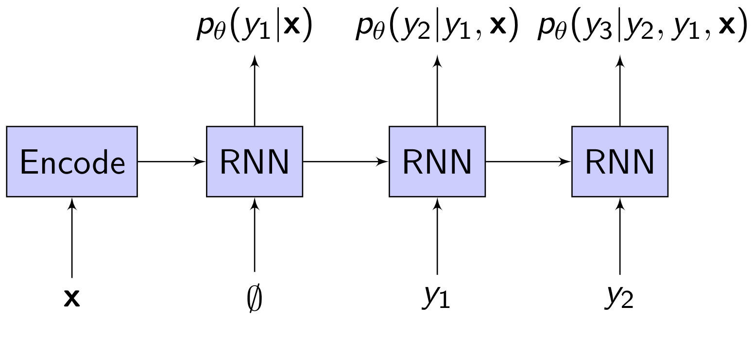
Hopefully, the encoding (a single vector) will contain all the information in the input needed for the decoder to accurately model the correct output. Then we just proceed to calculate $p_{\theta}(\mathbf{y}|\mathbf{x})$ as we would calculate $p_{\theta}(\mathbf{y})$, by multiplying the probabilities of all the $y_u$’s together:

Here’s a question you might ask, looking at the diagram of the model: Given that an RNN has state, and can remember what it has already outputted, why we do we need to feed $y_1, y_2, \dots$ into the decoder to compute the probability of the next output $y_u$?

There are two good reasons.

• First, if we don’t make the output explicitly conditioned on the previous outputs, we are implicitly saying that the outputs are independent, which may not be a good assumption. Consider transcribing a recording of someone saying “triple A”. There are two valid transcriptions: $\text{AAA}$ and $\text{triple A}$. If the first output $y_1$ is $\text{A}$, then we can be certain that the second output $y_2$ will be $\text{A}$.³

• Second, feeding in previous outputs allows us to use a feedforward model (which does not have state) for the decoder. A feedforward model can be much faster to train, since each $p_{\theta}(y_u|y_{u-1},y_{u-2},\dots,y_{1},\mathbf{x})$ term can be computed in parallel.⁴

Although we’ve been writing $p_{\theta}(\mathbf{y}|\mathbf{x})$, it’s usually better to work with the log probability $\text{log } p_{\theta}(\mathbf{y}|\mathbf{x})$ instead, for a few reasons. First, it is often easier to work with sums than it is to work with products. Recall that $\text{log }(a \cdot b) = \text{log }a + \text{log }b$. Thus, if you take the log of $p_{\theta}(\mathbf{y}|\mathbf{x})$, it becomes a sum instead of a product:

This prevents multiplying together a bunch of numbers smaller than 1, which could cause an underflow. It also makes training the model using gradient descent easier, since minimizing a sum of terms is easier than minimizing a product of terms.⁵ And finally, since many useful probability distributions have an $\text{exp}(\cdot)$ term (including softmax, Gaussian, and Poisson), and $\text{log }\text{exp}(a) = a$, taking the log may transform $p_{\theta}$ into a simpler form.

Learning

Now that we have a way of computing $p_{\theta}(\mathbf{y}|\mathbf{x})$ using a neural network, we need to train the model, i.e. find $\theta$ such that the model distribution $p_{\theta}(\mathbf{y}|\mathbf{x})$ matches the true distribution $p(\mathbf{y}|\mathbf{x})$. As usual with neural networks, we can do that by minimizing a loss function.

Many seq2seq papers don’t explicitly write out a loss function, though. Instead, they will just say something like “we use maximum likelihood” or “we minimize the negative log likelihood”. Here, we will see how this translates to a particular loss function that you can implement.

Suppose that you have a training set $\mathcal{T}$ composed of ($\mathbf{x}^i, \mathbf{y}^i$) pairs. If the training examples are considered to be fixed, and you think of $p_{\theta}(\mathbf{y}|\mathbf{x})$ as a function of the parameters $\theta$, then we call $p_{\theta}(\mathbf{y}^i|\mathbf{x}^i)$ the “likelihood” of the training example ($\mathbf{x}^i, \mathbf{y}^i$). In maximum likelihood estimation, the model parameters $\theta$ are learned by maximizing the likelihood of the entire training set, $L_{\theta}(\mathcal{T})$, which is the product of the likelihoods of all the training examples:

If these ($\mathbf{x}^i, \mathbf{y}^i$) samples are independent and identically distributed (i.i.d.), then as the number of samples increases, maximum likelihood estimation gives you a model that is closer and closer to the true distribution.

As mentioned earlier, it’s easier to maximize a sum than it is to maximize a product, so we take the log, and maximize that instead. (The log function is monotonic—that is, $\text{log }a > \text{log }b$ implies that $a > b$—so maximizing the log likelihood is equivalent to maximizing the likelihood.) Also, in machine learning it’s often more natural to think of minimizing a loss function, so we minimize the negative log likelihood:

If we expand the summed term, we get:

In other words, for every example in the dataset, we sum up the negative log probability of the correct output at each timestep, given the previous correct outputs.

Feeding the previous correct outputs into the model during training, as opposed to the model’s own predictions, is called “teacher forcing”. A long time ago (in deep learning years, which are like dog years), it was thought that teacher forcing is bad, and you should sometimes sample previous outputs from the model’s output distribution.⁶ Nowadays, this is less common, and big parallelizable seq2seq models like the Transformer⁷ rely on teacher forcing to go fast. Also, the name “teacher forcing” makes it sound like a hack, but really it’s the right way to apply maximum likelihood!

To minimize the negative log likelihood loss, you can use stochastic gradient descent (SGD), just like in a regular classification problem.

Inference

So far, we’ve described how you can use a neural network to compute $p_{\theta}(\mathbf{y}|\mathbf{x})$, and how to train the model using maximum likelihood.

The question remains: How do we generate an output? That is, how do we find $\underset{\mathbf{y}}{\text{argmax }} p_{\theta}(\mathbf{y}|\mathbf{x})$, given a new $\mathbf{x}$?

The brute force solution is an exhaustive search: just compute $p_{\theta}(\mathbf{y}|\mathbf{x})$ for every possible $\mathbf{y}$ and pick the $\mathbf{y}$ with the highest probability. That’s what exactly what we do for classification problems.

However, unlike a typical classification problem, where you might have a thousand classes, in any practical sequence prediction problem there will be astronomically many possible output sequences, so an exhaustive search is infeasible.

That means we need a new ingredient: an efficient search algorithm. The goal of the search is to approximately find $\mathbf{y}^* \approx \underset{\mathbf{y}}{\text{argmax }} p_{\theta}(\mathbf{y}|\mathbf{x})$.

(Note: for historical reasons⁸, the search process is also often called “decoding”. I’m not a big fan of this terminology because “decoding” already means several other things in machine learning.)

We will consider two search algorithms:

• greedy search
• beam search

1) Greedy search. A greedy search works as follows: at each step, pick the top output of the network, and feed this output back into the network. In other words, for each timestep $u$, pick $y_u^* = \underset{y_u}{\text{argmax }} p_{\theta}(y_u | y_{u-1}^*, y_{u-2}^*, \dots, y_{1}^*, \mathbf{x})$.

The search can continue until an “end-of-sequence” is predicted, or until a maximum number of steps has occurred. An example of a greedy search is shown in the diagram below:

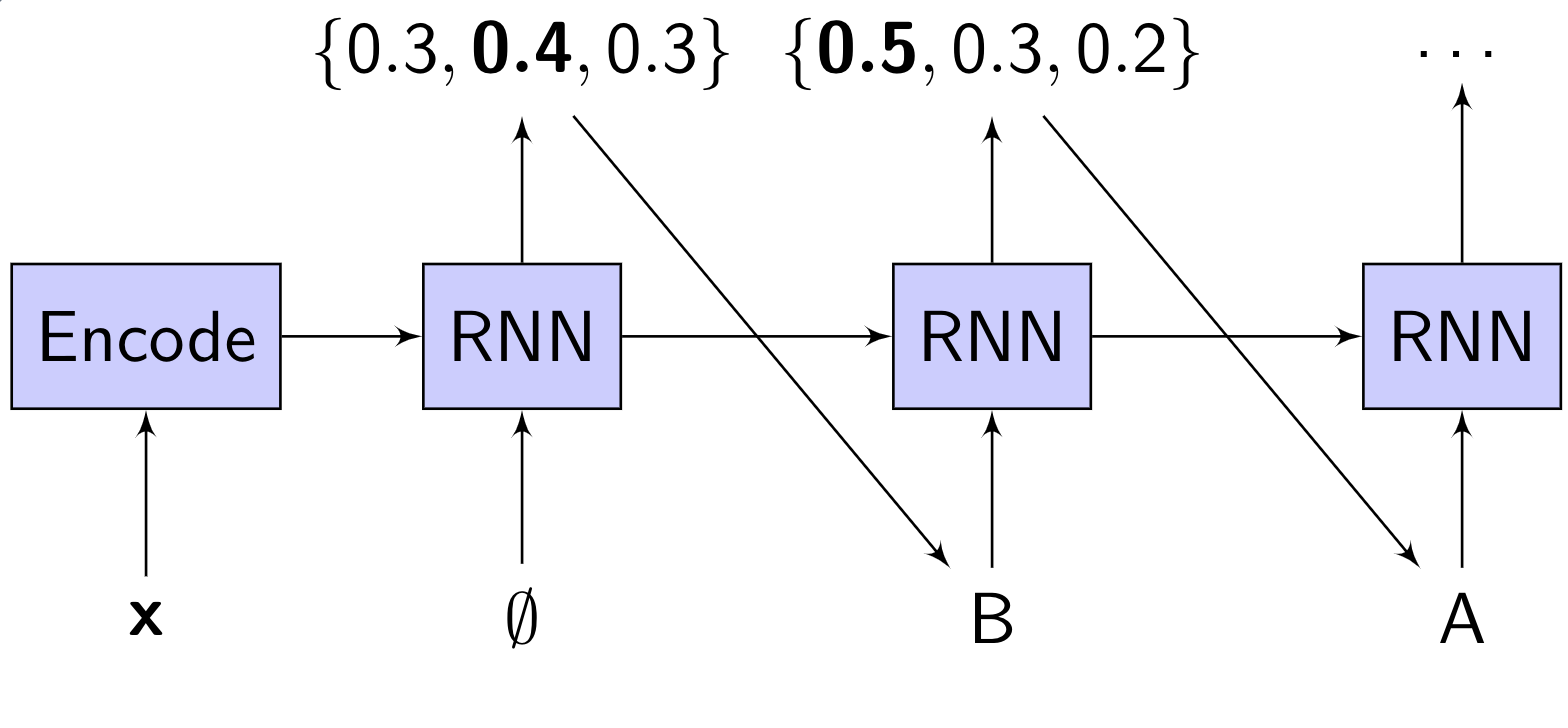
Because inference requires making a prediction, and feeding it back in to make the next prediction, this type of model is called “autoregressive” (“auto”=”self”, “regress”=”predict”).

2) Beam search. Greedy searching is fast, but you can show that it will not always find the most likely output sequence. As an example, suppose that:

• $p_{\theta}(a|\mathbf{x}) = 0.4$
• $p_{\theta}(b|\mathbf{x}) = 0.6$

and

• $p_{\theta}(aa|\mathbf{x}) = 0.4$
• $p_{\theta}(ab|\mathbf{x}) = 0.0$
• $p_{\theta}(ba|\mathbf{x}) = 0.35$
• $p_{\theta}(bb|\mathbf{x}) = 0.25$

Here, a greedy search would pick $b$, then $a$, and thus return $ba$, which has probability $0.35$. But the most likely sequence is actually $aa$, which has a probability of $0.4$.

We can get better results if we delay decisions about keeping a particular output until we have considered some future outputs. Beam search is one way of doing this.

In a beam search, we maintain a list (“beam”) of $B$ likely sequences (“hypotheses”). At each step, for each hypothesis, we compute the top $B$ outputs, and append them to the hypothesis. Now we have $B^2$ hypotheses. Of these, we prune the beam down to the top $B$, and then we continue to the next step.

An example of a beam search with $B=3$ is shown below.⁹

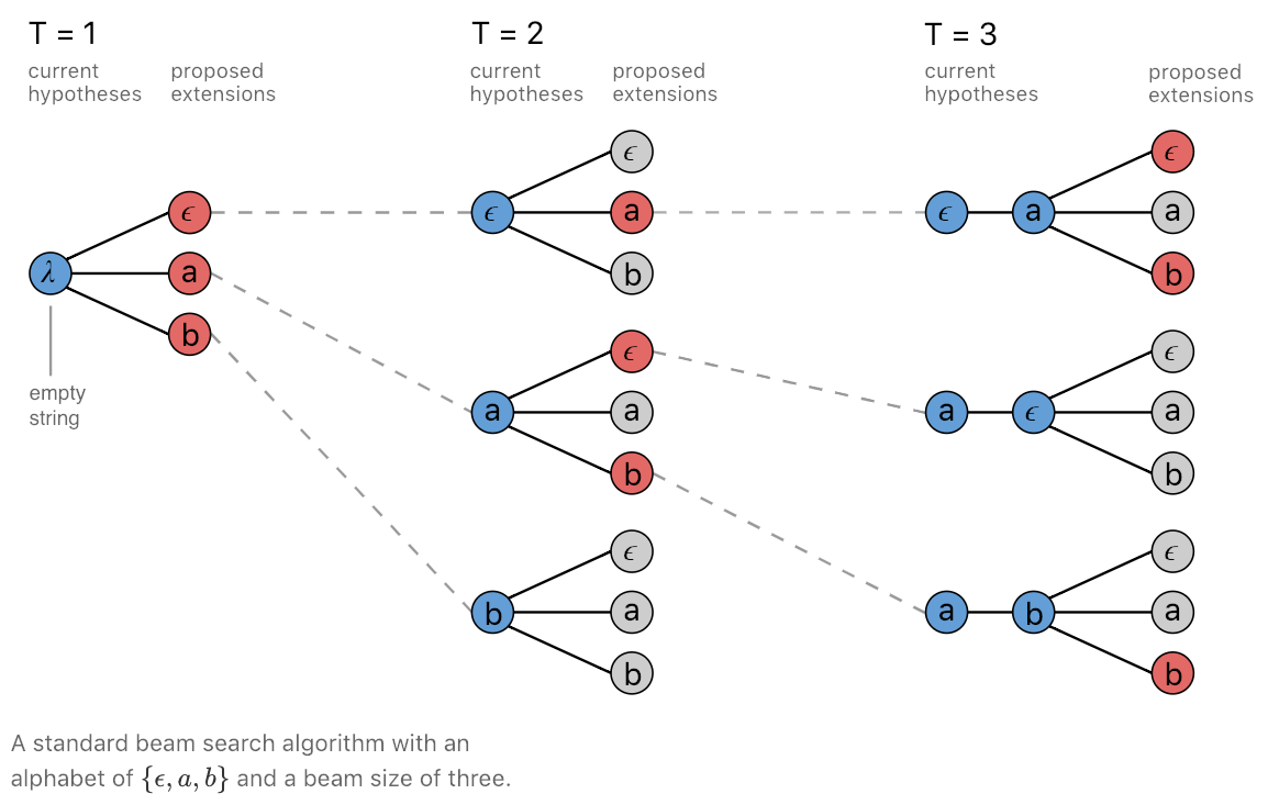
The algorithm returns the top $B$ hypotheses found. If your goal is just to estimate $\mathbf{y}$, you would just keep the top hypothesis, but for some applications it may also be useful to keep the rest of the hypotheses.

Notice that if $B = 1$, the beam search is equivalent to a greedy search. Also, if $B = \infty$, the beam search becomes an exhaustive search.

Beam search, too, is not guaranteed to find the most likely output sequence, but the wider you make the beam, the smaller the chance of a search error.¹⁰ The tradeoff is that you must re-run the neural network $B$ times, since you need to feed outputs back in.

Attention

We now have a complete method for doing sequence-to-sequence learning.

Unfortunately, if you apply the method exactly as described above—using an encoder RNN to map the input to a fixed-length vector consumed by the decoder RNN—it will not work for long sequences. The problem is that it is difficult to compress the entire input sequence into a single fixed-length vector.¹¹

Attention¹² is a mechanism that removes this fixed-length bottleneck. With attention, the decoder does not rely on a single vector to represent the input; instead, at every decoding step, it “looks” at a different part of the input using a weighted sum.

A more detailed introduction to the various forms of attention can be found here.

A toy task

Let’s use a toy task to test out our method. Consider the following string:

“Mst ppl hv lttl dffclty rdng ths sntnc”

This string is an example¹³ of how natural language is highly redundant or predictable: it’s generated by removing all the vowels from a normal sentence, and you can still understand the meaning.

If human intelligence can infer the missing vowels, then maybe artificial intelligence can as well! We will train a sequence-to-sequence model to take as input a vowel-less sentence (“Mst ppl”) and output the sentence with the correct vowels re-inserted (“Most people”).

This toy task is a bit easier to work with than a task like speech recognition or translation, in which you need lots of labelled data and lots of tricks to get something to work. A tutorial which covers the actual useful task of translating from French to English using PyTorch can be found here.

Running the experiment

We can easily generate a dataset for the task of inferring missing vowels using existing text. I used the text of “War and Peace”¹⁴: the input sequences are lines from the text with all the vowels removed, and the target output sequences are just the original lines. I also added the Penn Treebank (PTB) dataset, a commonly used dataset of news articles for language modeling experiments, to give the training data a little variety.

To run the code for yourself, or to train a model for filling in missing vowels on a new dataset, the code and a pre-trained model for this experiment can be found here.

We will first try training the simple encoder-decoder described above, without an attention mechanism. Here’s the result when we run a new sentence through the model:

input: Mst ppl hv lttl dffclty rdng ths sntnc.
truth: Most people have little difficulty reading this sentence.
guess: Mostov played with Prince Andrew and strengthers and

Oh dear! The search starts off strong—it correctly outputs “Most”—but then it gets distracted and tries to fill in the name “Rostov” (the name of a character in “War and Peace”). The next word, “played”, at least starts with the right letter, the “p” in “people”, but after that, the output really goes off the rails.

If we let the simple encoder-decoder model train a lot longer, the results get a bit better, but we still find bizarre mistakes like this:

input: th dy bfr, nmly, tht th cmmndr-n-chf
truth: the day before, namely, that the commander-in-chief
guess: the day before, manling that the mimicinacying Freemason

So let’s add in that fancy attention mechanism I mentioned and see if that helps:

input: Mst ppl hv lttl dffclty rdng ths sntnc.
truth: Most people have little difficulty reading this sentence.
guess: Most people have little difficulty riding this sentence.

Much better! But still not completely correct.

Let’s look at the beam (the $B$ hypotheses found by the beam search) and the beam scores (the hypotheses’ log probabilities):

Most people have little difficulty riding this sentence.   | -2.98
Most people have little difficulty reading this sentence.  | -3.28
Most people have little difficulty roading this sentence.  | -3.79
Most people have little difficulty riding those sentence.  | -3.81
Most people have little difficulty reading those sentence. | -4.11
Most people have little difficulty riding these sentence.  | -4.16
Most people have little difficulty reading these sentence. | -4.45
Most people have little difficulty roading those sentence. | -4.60

The correct answer does in fact appear in the beam (the 2nd hypothesis), but the model incorrectly assigns a higher probability to the hypothesis with “riding” instead of “reading”. Maybe with more/better training data this error would not occur, since “reading this sentence” ought to be a lot more probable in the training data than “riding this sentence”.

Notice another peculiar aspect of the beam: it is ordered (roughly) from shortest to longest. Autoregressive models are biased towards shorter output sequences!

Why? At each timestep, to compute the probability of a sequence, we multiply it (or add it, in the log domain) by the probability of the next output, which is always less than 1 (less than 0, in the log domain), so the probability of the complete sequence keeps getting smaller. In fact, the only thing keeping the search from producing outputs of length 0 is the fact that the model needs to predict the “end-of-sequence” token, and from the training data the model learns to assign low probability to “end-of-sequence” until it makes sense. It’s easy for the model to learn that a sentence like “The.” is very unlikely, but comparing two plausible sequences of roughly the same length seems to be harder.

How do people deal with the short-sequence bias in practice? Google Translate uses a variation¹⁵ of beam search in which the log probability is divided by a “length penalty” (“lp”), with a hyperparameter $\alpha$, that is computed as follows:

Yikes. How many TPU hours did they burn finding that formula? I hope we find a better way to mitigate the short-sequence bias!

The End

If you have any questions or if you find something wrong with this tutorial, please let me know.

Check out the code and try it out! It’s fun to feed the model random inputs, like your name, and see what stuff it comes up with trying to fill in the gaps. The code is also written in such a way that it should not be too hard to adapt it to a new task.

Thanks to Christoph Conrads and Mirco Ravanelli for their feedback on the draft of this post.